Elastic Frame Example
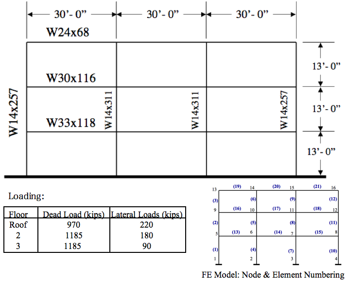
This example is of an elastic frame structure, as shown in the figure, subject to static loads. Here is the file: ElasticFrame.tcl
NOTE:
- The lines in the dashed boxes are lines that appear in the input file.
- all lines that begin with # are comments, they are ignored by the program (interpreter) but are useful for documenting the code. When creating your own input scripts you are highly encouraged to use comments.
- For brevity it is possible to put the comment after the command by using the ; to signify end of a command.
- The printing of info to the screen makes this example more complicated than it needs to be. If you don't understand it, you can ignore it for now.
Parameters
Before we build the model we are going to set some parameters using tcl variables and expression evaluation. We are going to set variables for PI, the gravtational constant g, and variables for each of our floor masses. We are using the tcl set and expr commands.
set PI  [expr 2.0 * asin(1.0)]
set g   386.4
set ft  12.0
set m1  [expr 1185.0/(4*$g)]; # 4 nodes per floor
set m2  [expr 1185.0/(4*$g)]
set m3  [expr  970.0/(4*$g)]
set w1  [expr 1185.0/(90*$ft)]
set w2  [expr 1185.0/(90*$ft)]
set w3  [expr  970.0/(90*$ft)]
Model
The model consists of sixteen nodes, twenty one elastic beam-column elements, a single load pattern with distributed loads, and constraints totally fixing the nodes at the base of the building. There are no material objects associated with the elastic elements, but there are geometric transformations. For this example all the columns have a PDelta transformation, and all the beams a linear transformation.
# Units: kips, in, sec
# Remove existing model
wipe

# Create ModelBuilder (with two-dimensions and 3 DOF/node)
model BasicBuilder -ndm 2 -ndf 3


# Create nodes & add to Domain -
# command: node nodeId xCrd yCrd <-mass $massX $massY $massRz>
#   NOTE: mass is optional
node 1     0.0   0.0
node 2   360.0   0.0
node 3   720.0   0.0
node 4  1080.0   0.0
node 5    0.0  162.0 -mass $m1 $m1 0.0
node 6  360.0  162.0 -mass $m1 $m1 0.0
node 7  720.0  162.0 -mass $m1 $m1 0.0
node 8 1080.0  162.0 -mass $m1 $m1 0.0
node 9     0.0 324.0 -mass $m2 $m2 0.0
node 10  360.0 324.0 -mass $m2 $m2 0.0
node 11  720.0 324.0 -mass $m2 $m2 0.0
node 12 1080.0 324.0 -mass $m2 $m2 0.0
node 13    0.0 486.0 -mass $m3 $m3 0.0
node 14  360.0 486.0 -mass $m3 $m3 0.0
node 15  720.0 486.0 -mass $m3 $m3 0.0
node 16 1080.0 486.0 -mass $m3 $m3 0.0

# Set the boundary conditions - command: fix nodeID xResrnt? yRestrnt? rZRestrnt?
fix 1 1 1 1
fix 2 1 1 1
fix 3 1 1 1
fix 4 1 1 1

# Define geometric transformations for beam-column elements
geomTransf Linear 1; # beams
geomTransf PDelta 2; # columns

# Define elements
# Create elastic beam-column elements -
# command: element elasticBeamColumn eleID node1 node2 A E Iz geomTransfTag

# Define the Columns
element elasticBeamColumn  1  1  5 75.6 29000.0 3400.0 2; # W14X257
element elasticBeamColumn  2  5  9 75.6 29000.0 3400.0 2; # W14X257
element elasticBeamColumn  3  9 13 75.6 29000.0 3400.0 2; # W14X257
element elasticBeamColumn  4  2  6 91.4 29000.0 4330.0 2; # W14X311
element elasticBeamColumn  5  6 10 91.4 29000.0 4330.0 2; # W14X311
element elasticBeamColumn  6 10 14 91.4 29000.0 4330.0 2; # W14X311
element elasticBeamColumn  7  3  7 91.4 29000.0 4330.0 2; # W14X311
element elasticBeamColumn  8  7 11 91.4 29000.0 4330.0 2; # W14X311
element elasticBeamColumn  9 11 15 91.4 29000.0 4330.0 2; # W14X311
element elasticBeamColumn 10  4  8 75.6 29000.0 3400.0 2; # W14X257
element elasticBeamColumn 11  8 12 75.6 29000.0 3400.0 2; # W14X257
element elasticBeamColumn 12 12 16 75.6 29000.0 3400.0 2; # W14X257

# Define the Beams
element elasticBeamColumn 13  5  6 34.7 29000.0 5900.0 1; # W33X118
element elasticBeamColumn 14  6  7 34.7 29000.0 5900.0 1; # W33X118
element elasticBeamColumn 15  7  8 34.7 29000.0 5900.0 1; # W33X118
element elasticBeamColumn 16  9 10 34.2 29000.0 4930.0 1; # W30X116
element elasticBeamColumn 17 10 11 34.2 29000.0 4930.0 1; # W30X116
element elasticBeamColumn 18 11 12 34.2 29000.0 4930.0 1; # W30X116
element elasticBeamColumn 19 13 14 20.1 29000.0 1830.0 1; # W24X68
element elasticBeamColumn 20 14 15 20.1 29000.0 1830.0 1; # W24X68
element elasticBeamColumn 21 15 16 20.1 29000.0 1830.0 1; # W24X68

# Create a Plain load pattern with a linear TimeSeries:
#  command pattern Plain $tag $timeSeriesTag { $loads }
pattern Plain 1 1 {
    eleLoad -ele 13 14 15 -type -beamUniform -$w1
    eleLoad -ele 16 17 18 -type -beamUniform -$w2
    eleLoad -ele 19 20 21 -type -beamUniform -$w3
}
Analysis - Gravity Load
We will now show the commands to perform a gravity load analysis. As the model is elastic we will use a Linear solution algorithm and use a single step of load control to get us to the desired load level.
# Create the system of equation
system BandSPD

# Create the DOF numberer, the reverse Cuthill-McKee algorithm
numberer RCM

# Create the constraint handler, a Plain handler is used as homo constraints
constraints Plain

# Create the integration scheme, the LoadControl scheme using steps of 1.0
integrator LoadControl 1.0

# Create the solution algorithm, a Linear algorithm is created
algorithm Linear

# create the analysis object
analysis Static
Perform The Gravity Analysis
After the objects for the model, analysis and output has been defined we now perform the analysis.
analyze 1
Print Info to Screen to Allow User to Check Results
In addition to using recorders, it is possible to specify output using the print and puts commands. When no file identifiers are provided, these commands will print results to the screen. We use the nodeReaction command to return the reactions at the individual nodes and the tcl lindex command to obtain the values from these lists.
# invoke command to determine nodal reactions
reactions

set node1Rxn [nodeReaction 1]; # nodeReaction command returns nodal reactions for specified node in a list
set node2Rxn [nodeReaction 2]
set node3Rxn [nodeReaction 3]
set node4Rxn [nodeReaction 4]

set inputedFy  [expr -$Load1-$Load2-$Load3]; # loads added negative Fy direction to ele
set computedFx [expr [lindex $node1Rxn 0]+[lindex $node2Rxn 0]+[lindex $node3Rxn 0]+[lindex $node4Rxn 0]]
set computedFy [expr [lindex $node1Rxn 1]+[lindex $node2Rxn 1]+[lindex $node3Rxn 1]+[lindex $node4Rxn 1]]

puts "\nEqilibrium Check After Gravity:"
puts "SumX: Inputed: 0.0 + Computed: $computedFx = [expr 0.0+$computedFx]"
puts "SumY: Inputed: $inputedFy + Computed: $computedFy = [expr $inputedFy+$computedFy]"
Add Lateral Loads
Now we prepare to add our lateral loads to the model. First we need to set the gravity loads acting constant, i.e. we do not want them changing as we apply more loads to the model. Then we will create load pattern with nodal loads to add to the model.
# set gravity loads constant and time in domain to 0.0
loadConst -time 0.0

timeSeries Linear 2
pattern Plain 2 2 {
    load 13 220.0 0.0 0.0
    load  9 180.0 0.0 0.0
    load  5  90.0 0.0 0.0
}
Recorder
We will create an element recorder to record the forces at the bottom story columns.
recorder Element -file eleForces.out -ele 1 4 7 10 forces
Perform The Lateral Load Analysis
After the objects for the model, analysis and output has been defined we now perform the analysis.
analyze 1
Print Info to Screen to Allow User to Check Results
In addition to using recorders, it is possible to specify output using the print and puts commands. When no file identifiers are provided, these commands will print results to the screen.
reactions

set node1Rxn [nodeReaction 1]; # nodeReaction command returns nodal reactions for specified node in a list
set node2Rxn [nodeReaction 2]
set node3Rxn [nodeReaction 3]
set node4Rxn [nodeReaction 4]

set inputedFx  [expr 220.0+180.0+90.0]
set computedFx [expr [lindex $node1Rxn 0]+[lindex $node2Rxn 0]+[lindex $node3Rxn 0]+[lindex $node4Rxn 0]]
set computedFy [expr [lindex $node1Rxn 1]+[lindex $node2Rxn 1]+[lindex $node3Rxn 1]+[lindex $node4Rxn 1]]

puts "\nEqilibrium Check After Lateral Loads:"
puts "SumX: Inputed: $inputedFx + Computed: $computedFx = [expr $inputedFx+$computedFx]"
puts "SumY: Inputed: $inputedFy + Computed: $computedFy = [expr $inputedFy+$computedFy]"

# print ele information for columns at bottom
print ele 1 4 7 19
Finally look at the eigenvalues
After the lateral load analysis has completed we will look at the period of the structure. To do this we use the eigenvalue command to obtain the eigenvalues. These are returned in a tcl list. From the list we obtain the eigenvalue for the mode using the tcl lindex command and use the expr command to determine the period.
set eigenValues [eigen 5]

puts "\nEigenvalues:"
set eigenValue [lindex $eigenValues 0]
puts "T[expr 0+1] = [expr 2*$PI/sqrt($eigenValue)]"
set eigenValue [lindex $eigenValues 1]
puts "T[expr 1+1] = [expr 2*$PI/sqrt($eigenValue)]"
set eigenValue [lindex $eigenValues 2]
puts "T[expr 2+1] = [expr 2*$PI/sqrt($eigenValue)]"
set eigenValue [lindex $eigenValues 3]
puts "T[expr 3+1] = [expr 2*$PI/sqrt($eigenValue)]"
set eigenValue [lindex $eigenValues 4]
puts "T[expr 4+1] = [expr 2*$PI/sqrt($eigenValue)]"

# create a recorder to record eigenvalues at all free nodes
recorder Node -file eigenvector.out -nodeRange 5 16 -dof 1 2 3 eigen 0

# record the results into the file
record
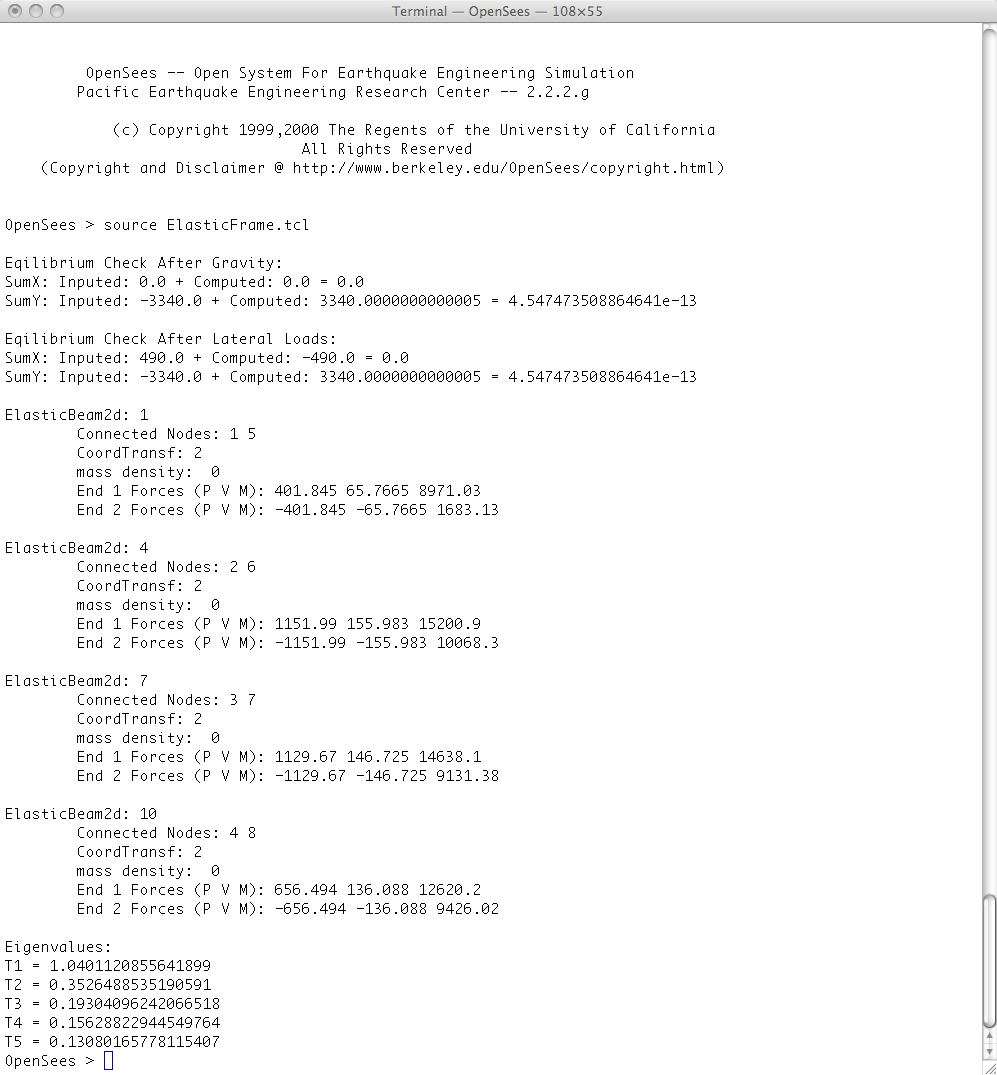
Results
When you run this script, you should see the following printed to the screen: