Flexure-Shear Interaction Displacement-Based Beam-Column Element

A beam-column element model that includes flexure and shear interaction was incorporated in OpenSees based on the work by Massone et al. (2006). The implementation was kept similar to existing elements, such that the modeling would keep familiar terms to currents users. To achieve that, an existing model was modified, as well as the section definition. The selected element model for modification is the displacement-based element which already included linear curvature and constant axial strain, but no shear deformation. The modifications were done at three levels: element formulation (fiber element), sectional analysis and fiber modeling. Additionally a new material model for concrete was introduced using the constitutive material laws described in this report with simple hysteretic rules.

1. FLEXURE-SHEAR INTERACTION MODEL

1.1 ELEMENT FORMULATION

In the original fiber element (Displacement-Based Beam-Column Element) implemented in OpenSees, based on linear interpolation of the curvature and constant axial strain, a third strain component was included to account for shear flexibility. The fiber discretization leads no longer to just uniaxial behavior, but rather a biaxial response by incorporating a membrane material model based on simple uniaxial stress-strain curves for concrete and steel. Although the material models can be cyclic, the element model formulation has been implemented and verified initially for monotonic static analysis. Details of the formulation can be found elsewhere (Massone et al., 2006; Massone 2006). The compatibility equations to relate nodal displacements (6 DOF) and internal strains (axial strain, curvature and shear strain) are defined only in a 2D plane, so that no 3D analysis is possible with this element. It also requires a specific geometric transformation called "LinearInt", which is based on the traditional geometric linear transformation, and therefore no other geometric transformation can be used.

The input parameters are the same as the original fiber element, however a new term, the location of the center of rotation (c), is required to distribute transversal displacement between flexural (curvature) and shear (shear strain) components. This parameter is defined as the fraction of the element height (measured from top) that corresponds to the center of curvature.

Flexure-Shear Interaction Displacement-Based Beam-Column Element

This command is used to construct a dispBeamColumnInt element object, which is a distributed-plasticity, displacement-based beam-column element which includes interaction between flexural and shear components.

element dispBeamColumnInt $eleTag $iNode $jNode $numIntgrPts $secTag $transfTag $cRot <-mass $massDens>

The valid queries to a displacement-based beam-column element when creating an ElementRecorder object are 'force,' 'stiffness,' and 'section $secNum secArg1 secArg2...' Where $secNum refers to the integration point whose data is to be output. It also requires a specific geometric transformation called "LinearInt", which is based on the traditional geometric linear transformation, and therefore no other geometric transformation can be used.

Example:

geomTransf LinearInt 1

element dispBeamColumnInt 1 1 3 2 2 1 0.4

1.2 SECTIONAL ANALYSIS

The section formulation required for each element is based also on a similar formulation implemented in OpenSees. However, not all capabilities are included as in the original formulation. The section is defined as a fiber section, but based only in fiber components and not in patch or layer components for simplicity. It has been formulated in this way to make sure that the strip modeling is understood since differently to the standard fiber section analysis the strips in the model with interaction between shear and flexure requires that all the strips are formed with smeared (average) concrete and reinforcement areas.

The definition of the fiber section is initiated by establishing in the heading of the command the thickness of the section (three in this case to represent boundary elements). The thickness of the element is required to verify equilibrium in the horizontal direction (assuming that same area ratio holds between concrete materials inside a strip in horizontal and vertical directions). For generality, the section is allowed to have three different thicknesses to be able to model barbell or T-shaped walls (Fig. 1). Each thickness may be associated to several strips.

Strips are created from concrete and steel materials. Since the strip unit corresponds to the membrane (panel) element, the location of each of them is defined by the fiber coordinate ($yLoc), and therefore, tributary concrete and steel areas inside each strip are located at one same point (Fig. 1). This may difficult the analysis, but the model is based on uniform (smeared) steel and concrete distribution. Even though a center of area (concrete and steel) defined by using a transformed area for steel may be acceptable, in tensile governed elements a better approximation may be using the steel location. For simplicity, the center of area of concrete may be selected for calculations, regarding a reasonable small strip size selection. In the fiber section definition, each strip is defined by fibers with same coordinate, and strips are organized from negative to positive location. Therefore all steel and concrete components of one strip have to be together (one after the other). The change in fiber location tells the program that a different strip is initiated. To complete the strip definition, the horizontal steel reinforcement has to be included. The steel is assumed uniformly distributed in the section, so that it may be located as only one fiber (recommended). In the case of horizontal steel, the component is called as "Hfiber" and the area defined in such fiber corresponds to the total horizontal steel area in one single element (for the entire element). This steel is assumed to be the same for all strips inside the section.

For consistency when defining the fiber section, the command requires to define the number of strips within each sub-section with the same thickness, which has to add up the same number of different fiber locations defined in the section (total number of strips).

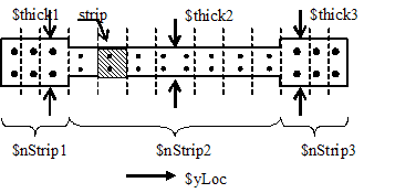
Fig. 1 Element section modeling.

The original uniaxial definition of the fiber components inside the fiber section recorded only uniaxial stresses and strains for the fiber, and resultant axial force, moment, axial strain and curvature for the section. In the membrane (panel) formulation for the strips, other quantities may be useful to record. At the strip level new recorders have been included: eX (horizontal strain), eY (axial strain), e1 (principal strain in direction 1), e2 (principal strain in direction 2), alpha (angle for principal axis, measured counterclockwise from eY to e1), sX (average horizontal steel stress), sY (average vertical steel stress), s1 (average principal concrete stress in direction 1) and s2 (average principal concrete stress in direction 2). The mentioned recorders are called by sections, so that the output gives the results organized in columns for each strip inside the section, using the same order defined in the fiber section. At the section level, axial strain, curvature, shear strain, resultant axial force, moment and shear force are obtained with the standard recorder forceAndDeformation.

Example:

recorder Element -file Sect_eX.out -ele 1 section 1 eX

recorder Element -file Sect_s2.out -ele 1 section 1 s2

Fiber Section for Interaction Model

The FiberInt object is composed of Fiber objects (fiber and Hfiber). Individual fibers are defined using the fiber command (concrete or vertical steel) or Hfiber (horizontal steel) command. During generation, the Fiber objects are associated with uniaxialMaterial objects. The geometric parameters are defined with respect to a planar local coordinate system (y,z).

section FiberInt $secTag -NStrip $nStrip1 $thick1 $nStrip2 $thick2 $nStrip3 $thick3 {

fiber <fiber arguments> # same as for section Fiber

Hfiber <fiber arguments>

}

Example:

section FiberInt 2 –NStrip 1 6.5 1 2.0 1 6.5 {

fiber -25.55 0 15.6 2

fiber -25.55 0 1.24 1003

fiber 0 0 35.6 2

fiber 0 0 0.84 1003

fiber +25.55 0 15.6 2

fiber +25.55 0 1.24 1003

Hfiber 0 0 0.0718 1005

}

1.3 FIBER MODELING – MATERIAL MODELING

As described previously, the section is created based on strips, and each strip consists of vertical fibers (fiber) that represent steel and concrete materials and horizontal fibers (Hfiber) that represent the horizontal steel. Since uniform distribution of reinforcement steel is assumed at strip level, all horizontal steel reinforcement can be included as only one horizontal fiber. The location of such fiber is included in the command just for completeness, but it is not necessary for any calculation. The area required in the Hfiber corresponds to the total steel tributary area present in the element that holds the defined section. The internal numerical scheme defined to achieve equilibrium handles two different types of materials: steel and concrete. Since different steel and concrete stress-strain laws can be implemented and used with this model, the program needs to distinguish between concrete and steel. For simplicity, it has been selected the material tag ($matTag) to define whether a material is concrete or steel. Concrete materials are defined as materials with tag number under (or equal to) 1000 and steel materials use tag numbers over 1000 (see example).

HFiber Command

This command is used to construct a UniaxialFiber object and add it to the section as the steel horizontal component.

Hfiber $yLoc $zLoc $A $matTag

Example:

uniaxialMaterial Concrete01 2 -3 -0.002 0 -0.01

uniaxialMaterial Steel02 1003 60 29000 0.02 20 0.9 0.2 0 0.1 0 0.1

uniaxialMaterial Steel02 1005 60 29000 0.02 20 0.9 0.2 0 0.1 0 0.1

.

.

.

fiber -25.55 0 15.6 2 # vert. concrete

fiber -25.55 0 1.24 1003 # vert. steel

Hfiber 0 0 0.0718 1005 # horz. steel

Note: concrete materials are defined as materials with tag number under (or equal) 1000 and steel materials use tag numbers over 1000 (see example).

2. CONCRETE MATERIAL – CONCRETE06

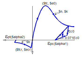
The concrete material, Concrete06 (Fig. 2), keeps the simplicity of previous formulations (Concrete01 to Concrete03). However, envelope curves have been modified to represent concrete behavior in membrane elements. Compressive constitutive material law (?c-?c) is defined as the Thorenfeldt-base curve, which is similar to Popovic (1973) definition:

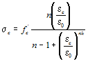(1)

where f'c is the compressive strength, ?0 is the strain at peak compressive stress, and n and k are parameters.

The tensile envelope uses the tension stiffening equation by Belarbi and Hsu (1994) with a general exponent b.

(2)

where fcr is the tensile strength, ?cr is the strain at tensile strength and b is a parameter.

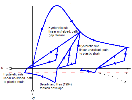
Fig. 2 General Concrete06 stress-strain law description (tension not to scale)

Hysteretic rules in compression are held similarly as defined in Concrete03, with linear unloading and reloading paths (constant stiffness). The unloading and reloading paths in compression are connected through unloading/reloading paths with initial elastic stiffness (Fig. 2 and 3). The unloading path in compression has a stiffness of 7.1% of the initial elastic stiffness (0.071Ec) as adopted by Palermo and Vecchio (2003). The plastic compressive strain (?pc), defined as the residual unrecoverable compressive strain obtained after full unloading (zero stress) is characterized by:

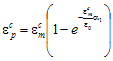(3)

where ?mc is the maximum (absolute value) compressive strain attained previously on the envelope (stored value by the uniaxial material), and ?1 is a parameter.

A origin-oriented hysteretic rule for tension may introduce inaccuracies in the analysis. In this case, stresses are linear and recover the initial strain (from previous cycle) when reducing to zero. However, after opening of cracks, under unloading from tension, the uneven and rough surface of the crack tend to initiate contact before the initial strain from previous cycle is attained. This effect known as gap closure improves the dissipating characteristic of the hysteretic rule, reducing the pinching. For this reason, the hysteretic rule for concrete in tension in this model considers a plastic strain (different from zero or the strain from previous cycle) such that when going from tensile stresses to compressive stresses the gap closure effect is modeled by a linear path. Such consideration requires also keeping track of previous stiffness and maximum tensile stress, and the previous tensile plastic strain. This is required, since when going in a posterior cycle from compressive stresses to tensile stresses the compressive plastic strain will become the new origin of the tensile behavior, creating a shifting in the stress-strain curve in tension (Fig. 3). From that strain a linear path will be followed using the previous unloading stiffness in tension until the previous attained maximum tensile stress is reached.

In tension, the unloading and reloading paths are the same, and are defined by the tensile plastic strain (?pt). A similar equation is used to characterize the tensile plastic strain as in compression:

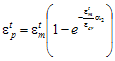(4)

where ?mt is the maximum tensile strain attained previously on the envelope (stored value by the uniaxial material), and ?2 is a parameter.

Even though the equation for plastic strain (tension or compression) can be generally used, an internal checking is included in the model such that the unloading/reloading paths have as maximum stiffness the initial stiffness.

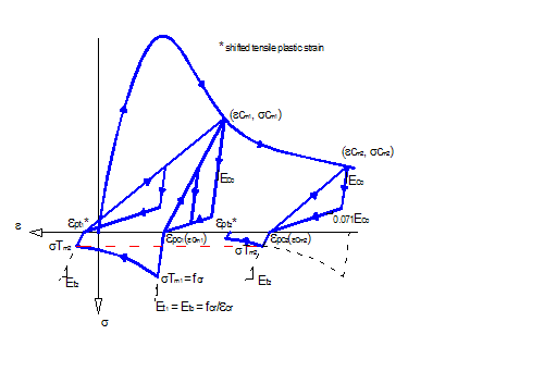
Fig. 3 Variables in Concrete06 stress-strain law (tension not to scale)

Concrete06 Material

This command is used to construct a uniaxial concrete material object with tensile strength, nonlinear tension stiffening and compressive behavior based on Thorenfeldt curve.

uniaxialMaterial Concrete06 $matTag $fc $e0 $n $k $alpha1 $fcr $ecr $b $alpha2

*NOTE: Compressive concrete parameters should be input as negative values.

Example:

uniaxialMaterial Concrete06 1 -3 -0.002 2 1 0.32 0.3 0.00008 4 0.08

3. REFERENCES

3.1 FLEXURE-SHEAR INTERACTION MODEL

1. Massone, L. M., 2006; "RC Wall Shear – Flexure Interaction: Analytical and Experimental Responses", Ph.D. Dissertation, University of California, Los Angeles, June 2006, 398 pp.

2. Massone, L. M.; Orakcal, K.; and Wallace, J. W. , 2006; "Shear - Flexure Interaction for Structural Walls"; SP-236, ACI Special Publication – Deformation Capacity and Shear Strength of Reinforced Concrete Members Under Cyclic Loading, editors: Adolfo Matamoros & Kenneth Elwood, p. 127-150.

3.2 CONCRETE06 MODEL

1. Popovics, S., 1973, "A Numerical Approach to the Complete Stress-Strain Curve of Concrete", Cement and Concrete Research, V. 3, No. 4, pp. 583-599.

2. Belarbi, H. and Hsu, T.C.C., 1994, "Constitutive Laws of Concrete in Tension and Reinforcing Bars Stiffened by Concrete", ACI Structural Journal, V. 91, No. 4, pp. 465-474.

3. Palermo, D., and Vecchio, F. J., 2003, "Compression Field Modeling of Reinforced Concrete Subjected to Reversed Loading: Formulation", ACI Structural Journal, V. 100, No. 5, pp. 616 - 625.

4. WALL01-EXAMPLE

The following example creates a wall model formed with 8 elements, where each element consists of 8 strips. The model represents a wall with a constant axial load and a variable lateral load applied at the top. It is considered fixed to the bottom and the lateral load is incremented trough prescribed displacements at wall top up to 1.6 in.

wipe; model basic -ndm 2 -ndf 3

set tolAx 1.0e-3; set iterAx 100;

set tolLatNew 1.0e-6; set iterLatNew 100;

set tolLatIni 1.0e-5; set iterLatIni 1000;

set dUi 0.02; # Displacement increment

set maxU 1.6; # Max. Displacement

#concrete parameters

set fc -6.21; set eo -0.0021; set r 2.91;

set k 1.36; set alphaC 0.32; set fcr 0.294;

set ecr 0.00008; set b 0.4; set alphaT 0.08;

set fcc -6.91; set ecc -0.0038; set rcc 1.88;

#steel parameters

set fyRed 59.15; set by 0.02; set Ry 1.564;

set roy 0.00327; set fyBRed 57.33; set byB 0.02;

set RyB 25.0; set royB 0.0293; set fxRed 59.15;

set bx 0.02; set Rx 1.564; set rox 0.00327;

#concrete (confined and unconfined)

uniaxialMaterial Concrete06 1 $fcc $ecc $rcc 1 $alphaC $fcr $ecr $b $alphaT;

uniaxialMaterial Concrete06 2 $fc $eo $r $k $alphaC $fcr $ecr $b $alphaT;

# steel (bound., web and horiz. reinforcement)

set E 29000.0;

uniaxialMaterial Steel02 1003 $fyBRed $E $byB $RyB 0.9 0.1 0 0.1 0 0.1 ;

uniaxialMaterial Steel02 1004 $fyRed $E $by $Ry 0.9 0.1 0 0.1 0 0.1 ;

uniaxialMaterial Steel02 1005 $fxRed $E $bx $Rx 0.9 0.1 0 0.1 0 0.1 ;

# Define cross-section

set t1 6.0; set NStrip1 2; # thickness 1

set t2 4.0; set NStrip2 4; # thickness 2

set t3 6.0; set NStrip3 2; # thickness 3

geomTransf LinearInt 1

set np 1; # int. points

set C 0.4; # center of rotation

#section definition

section FiberInt 2 -NStrip $NStrip1 $t1 $NStrip2 $t2 $NStrip3 $t3 {

#vertical fibers

fiber -23 1 10 1; fiber -23 1 5 2; fiber -23 1 0.3 1003;

fiber -19 1 10 1; fiber -19 1 5 2; fiber -19 1 0.3 1003;

fiber -14 1 33 2; fiber -14 1 0.1 1004;

fiber -6 1 33 2; fiber -6 1 0.1 1004;

fiber 6 1 33 2; fiber 6 1 0.1 1004;

fiber 14 1 33 2; fiber 14 1 0.1 1004;

fiber 19 1 10 1; fiber 19 1 5 2; fiber 19 1 0.3 1003;

fiber 23 1 10 1; fiber 23 1 5 2; fiber 23 1 0.3 1003;

#horiz. reinf.

Hfiber 0 0 0.2 1005;

}

#nodes

set n 8

node 1 0 0.0; node 2 0 160; node 3 0 20; node 4 0 40;

node 5 0 60; node 6 0 80; node 7 0 100; node 8 0 120; node 9 0 140;

#element definition

element dispBeamColumnInt 1 1 3 $np 2 1 $C

element dispBeamColumnInt 2 3 4 $np 2 1 $C

element dispBeamColumnInt 3 4 5 $np 2 1 $C

element dispBeamColumnInt 4 5 6 $np 2 1 $C

element dispBeamColumnInt 5 6 7 $np 2 1 $C

element dispBeamColumnInt 6 7 8 $np 2 1 $C

element dispBeamColumnInt 7 8 9 $np 2 1 $C

element dispBeamColumnInt 8 9 2 $np 2 1 $C

fix 1 1 1 1

# Set axial load

pattern Plain 1 Constant {

load 2 0.0 -85 0.0

}

initialize; integrator LoadControl 0 1 0 0;

system SparseGeneral -piv; test NormUnbalance $tolAx $iterAx 0;

numberer Plain; constraints Plain;

algorithm ModifiedNewton -initial; analysis Static;

# perform the gravity load analysis,

analyze [expr 1]

# Set the gravity loads to be constant & reset the time in the domain

loadConst -time 0.0

remove recorders

# set lateral load

pattern Plain 2 Linear {

load 2 1.0 0.0 0;

}

system BandGeneral; constraints Transformation; numberer Plain;

# Create a recorder to monitor nodal displacement and element forces

recorder Node -file nodeTop.out -node 2 -dof 1 disp

recorder Element -file elesX.out -time -ele 1 globalForce

# recorder for element1 section1 steel stress/strain and section force-def.

recorder Element -file Sect_FandD.out -ele 1 section 1 forceAndDeformation

recorder Element -file Sect_eX.out -ele 1 section 1 eX

recorder Element -file Sect_eY.out -ele 1 section 1 eY

recorder Element -file Sect_sX.out -ele 1 section 1 sX

recorder Element -file Sect_sY.out -ele 1 section 1 sY

test NormDispIncr $tolLatNew $iterLatNew;

algorithm ModifiedNewton -initial

analysis Static

set dU $dUi;

set numSteps [expr int($maxU/$dU)];

integrator DisplacementControl 2 1 $dU 1 $dU $dU

#source cycle2.tcl

#### end

set ok [analyze $numSteps]; set jump 1;

if {$ok != 0} {

set currentDisp [nodeDisp 2 1]

set ok 0

while {abs($currentDisp) < abs($maxU)} {

set ok [analyze 1]

puts "\n Trying.. $currentDisp\n"

# if the analysis fails try initial tangent iteration

if {$ok != 0} {

puts "\n regular newton failed .. try an initial stiffness"

test NormDispIncr $tolLatIni $iterLatIni 0;

algorithm ModifiedNewton -initial ;

set ok [analyze 1]

puts "\n Trying.. $currentDisp\n"

if {$ok == 0} {

puts " that worked .. back to regular newton \n"

set jump 1

integrator DisplacementControl 2 1 $dU 1

} else {

puts "\n that didn't worked .. Try next point\n"

set jump [expr $jump+1];

integrator DisplacementControl 2 1 [expr $dU*$jump] 1

}

test NormDispIncr $tolLatNew $iterLatNew

algorithm Newton

} else {set jump 1

integrator DisplacementControl 2 1 $dU 1

}

set currentDisp [expr $currentDisp+$dU]

}

}

#### end

The load-displacement obtained from the previous model is shown in Fig. 4 only for references.

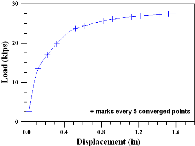
Fig. 4 Load-displacement response of example Wall01