Basic Truss Example
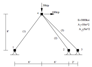
This example is of a linear-elastic three bar truss, as shown in the figure, subject to static loads. Here is the file: Truss.tcl
NOTE:
- The lines in the dashed boxes are lines that appear in the input file.
- all lines that begin with # are comments, they are ignored by the program (interpreter) but are useful for documenting the code. When creating your own input scripts you are highly encouraged to use comments.
Model
The model consists of four nodes, three truss elements, a single load pattern with a load acting at node 4, and constraints fixing the movement at the other three nodes in the model. As each Truss element has the same Young's Modulus, a single elastic material is created.
# units: kip, in

# Remove existing model
wipe

# Create ModelBuilder (with two-dimensions and 2 DOF/node)
model BasicBuilder -ndm 2 -ndf 2

# Create nodes
# ------------
# Create nodes & add to Domain - command: node nodeId xCrd yCrd
node 1   0.0  0.0
node 2 144.0  0.0
node 3 168.0  0.0
node 4  72.0 96.0

# Set the boundary conditions - command: fix nodeID xResrnt? yRestrnt?
fix 1 1 1
fix 2 1 1
fix 3 1 1

# Define materials for truss elements
# -----------------------------------
# Create Elastic material prototype - command: uniaxialMaterial Elastic matID E
uniaxialMaterial Elastic 1 3000

#
# Define elements
#

# Create truss elements - command: element truss trussID node1 node2 A matID
element Truss 1 1 4 10.0 1
element Truss 2 2 4 5.0 1
element Truss 3 3 4 5.0 1

# Define loads
# ------------
#

# create a Linear TimeSeries with a tag of 1
timeSeries Linear 1

# Create a Plain load pattern associated with the TimeSeries,
# command: pattern Plain $patternTag $timeSeriesTag { load commands }

pattern Plain 1 1 {

   # Create the nodal load - command: load nodeID xForce yForce
   load 4 100 -50
}
Analysis
We will now show the commands to perform a static analysis using a linear solution algorithm The model is linear, so we use a solution Algorithm of type Linear. Even though the solution is linear, we have to select a procedure for applying the load which is called an Integrator. For this problem, a LoadControl integrator advances the solution. The equations are formed using a banded system so the System is BandSPD, banded symmetric positive definite This is a good choice for most small size models. The equations have to be numbered so the widely used RCM (Reverse Cuthill-McKee) numberer is used. The constraints are most easily represented with a Plain constraint handler. Once all the components of an analysis are defined, the Analysis object itself is created. For this problem, a Static Analysis object is used.
# Create the system of equation
system BandSPD

# Create the DOF numberer, the reverse Cuthill-McKee algorithm
numberer RCM

# Create the constraint handler, a Plain handler is used as homo constraints
constraints Plain

# Create the integration scheme, the LoadControl scheme using steps of 1.0
integrator LoadControl 1.0

# Create the solution algorithm, a Linear algorithm is created
algorithm Linear

# create the analysis object
analysis Static
Output Specification
For this analysis, we will record the displacement at node 4, and all the element forces expressed both in the global coordinate system and the local system.
# create a Recorder object for the nodal displacements at node 4
recorder Node -file example.out -time -node 4 -dof 1 2 disp

# create a Recorder for element forces, one for global system and the other for local system
recorder Element -file eleGlobal.out -time -ele 1 2 3 forces
recorder Element -file eleLocal.out  -time -ele 1 2 3 basicForces
Perform The Analysis
After the objects for the model, analysis and output has been defined we now perform the analysis.
analyze 1
Print Information to Scree
In addition to using recorders, it is possible to specify output using the print and puts commands. When no file identifiers are provided, these commands will print results to the screen.
puts "node 4 displacement: [nodeDisp 4]"
print node 4
print element
Results
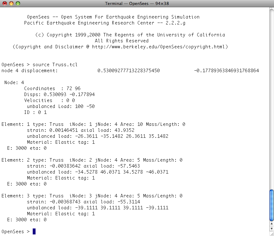
When you run this script, you should see the following printed to the screen:
In addition, your directory should contain the following 3 files with the data shown: